Theory of Operation
When a genome is sequenced and aligned against a reference, a number of portions of the DNA can vary drastically vary from the reference - this can be due to normal variations in DNA between individuals, or due to substantial variations such as caused by genetic diseases or cancer.
One potential structural variation can be that a region of DNA is either duplicated (potentially multiple times) or deleted from one or both copies of a chromosome, resulting in Copy Number Variations. When the size of the region which has been duplicated or deleted is shorter than the length of the reads used to perform the sequencing, this difference can be resolved by the alignment tool. If, however, the anomalous region is larger than the average read size, then the tools will instead register this as a variation in coverage, with only the (small number of) reads which cross the boundary between copies being evidence to the contrary.
The image below shows how an increase in coverage is evidence of a duplicated region with respect to the reference.
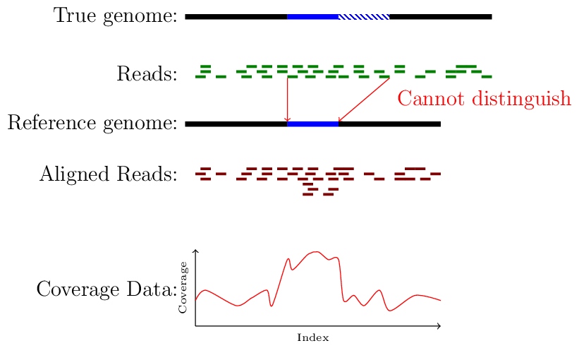
A demonstration of coverage-aliased copy numbers
The Challenge
A given coverage file is, however, extremely noisy, even when using high-fidelity long read platforms. Whilst the human eye can pick out certain large scale patterns on a chromosomal scale, the exact criteria for what can be considered a genuine CNV and what is merely noise can be somewhat difficult to distinguish.
One potential solution would be to pass a basic smoothing filter over the coverage data, thereby “denoising” it.
However, a smoothing operation is in fact antithetical to what we are attempting to find, which is sharp transition edges between regions of different multiplicity. A smoothing kernel, by definition, obscures those edges and can entirely eliminate smaller scale transitions should the smoothing length scale be larger than the length scale over which multiplicity can vary.
The Deforester tool is a method by which these transition edges can be located, without smoothing out all of the information of interest.
Underlying Theory
The Deforester tool (so named because it reduces the “forest” of coverage data into a singular “tree”) works on a series of successive Bayesian Inferences. Bayes’ Theorem says that, given data \(D\), a hypothesis \(H_1\) is better than the hypothesis \(H_2\) if it meets the criteria:
\[\frac{p(D | H_1) \text{prior}(H_1)}{p(D|H_2) \text{prior}(H_2)} > 1\]For convenience, we often work in logarithmic space, in which case the relationship is more easily expressed as:
\[\mathfrak{p}(D|H_1) + \log(\text{prior}(H_1) > \mathfrak{p}(D|H_2) + \log(\text{prior}(H_2)\]Where \(\mathfrak{p}\) is the log-probability of observing the data if the hypothesis were true, and \(\text{prior}(H)\) is the prior probability we have that \(H\) is true, before we looked at the data.
Algorithmic Overview
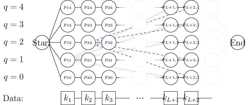
A demonstration of the network-based approach
First, compute the most likely value of the hyperparameters of the model (\(\gamma, \sigma, \nu\))
- Generate a layered network, where each layer corresponds to a given base, and each node in the layer corresponds to a given value of \(q\)
A node \(n_{iq}\) is associated with base \(i\) having mean coverage \(q\nu\)
- From the node \(n_{iq}\), you can travel to either \(n_{i+1,q}\) or \(n_{i+L,p\neq q}\)
The vertex \(n_{iq} \to n_{i+1q}\) has cost \(\mathfrak{p}(k_{i+1} = q | \gamma,\sigma,\nu)\)
The vertex \(n_{iq} \to n_{i+L,p\neq q}\) costs:
\(\sum_{j=i+1}^{i+L}\mathfrak{p}(k_{j} = p | \gamma,\sigma,\nu) + \text{Prior}(\text{jump})\)
Compute the minimal path through this network
Convert this path back into coverage/harmonic space
The “jump” vertices are a consequence of our prior which (as we shall see) dictates that we should only consider a transition if it is of sufficient length. This design element is hard-coded into our network.
Statistical Model
In order to generate the costs of the vertices, we must therefore formulate a statistical model and aggregate the knowledge that we have about our system. The following are the basic principles upon which Deforester operates:
The genome is sampled to a given average depth across all chromosomes, termed the fundamental frequency, and denoted \(\nu\). We assume that we know this in advance (in practice, we compute the most likely value).
- Every section of the genome has a given multiplicity, harmonic or resonance, denoted \(q\) - this is our estimation of the copy-number.
A region with an unresolved CNV is sampled to a depth of \(q\nu\).
Most portions of the human genome should have \(q = 2\), due to diploidy
- The sampling process is noisy
For each sampling depth, the process is distributed according to a Poisson distribution with mean \(\lambda\)
Variations in sampling mean that \(\lambda\) varies across the genome. We assume this is random and Gamma-distributed such that the mean \(\bar{\lambda} = \nu\), with standard deviation \(\sigma\)
There are then errors due to misalignment etc (this causes regions with true-coverage of zero to have small segments aligned to them, for example). We assume this error is Gaussian with standard deviation \(\gamma\)
The noise is distributed according to the standard iid assumptions
Deviations in \(q\) must be on a large scale (else they would have been resolved) - \(q\) should vary only over regions greater than a lengthscale \(L\).
If index \(i\) has \(q_i\), then we need a significant amount of evidence that \(q_{i+1} \neq q_i\).
The result of the above is that the probability that the component at base \(i\) was generated due to the \(q^\text{th}\) resonance is given by:
\[\begin{split}p(q_i = q | k_i, \nu, \sigma,\gamma) &= \sum_{k=0}^\infty N(k;k_i,\gamma) \int_0^\infty \text{Poisson}(k;\lambda) \Gamma(\lambda; q\nu, \sigma) \mathrm d \lambda \\ &= \sum_{k=0}^\infty N(k;k_i,\gamma) \times NB\left(k; \frac{q^2 \nu^2}{\sigma^2}, \frac{q\nu}{q \nu + \sigma^2}\right)\end{split}\]Where we have used the notation that \(N(k;\mu,\sigma)\) is the usual normal distribution probability given mean \(\mu\) and variance \(\sigma^2\), and \(\text{Poisson}(k;\lambda)\) is the usual Poisson probability of observing an integer event \(k\) given an average rate \(\lambda\) and \(\Gamma(\lambda,\mu,\sigma)\) is the Gamma distribution (expressed in terms of its first and second moments, instead of the standard notation). In the second line we used the property that the Gamma distribution is the conjugate prior of the Poisson distribution, with the result being the Negative Binomial distribution, \(NB(k;\mu,\sigma)\).
This is a function which we can precompute for a suitable range of \(k\) and \(q\) to be reused across the entire genome.
The quantity of interest for us is the value of *q*, which corresponds to the most likely multiplicity of any base, since *q* is constrained to be an integer: our goal is to find the most likely value of *q* for each base in the dataset
Since we are using the standard iid assumptions, the probability that a sequence of bases between \(i\) and \(j\) was generated on the \(q^\text{th}\) harmonic (i.e. in a region with multiplicity \(q\)), is:
\[\mathfrak{p}(q_{i \to j} = q | \{k_n\}, \nu, \sigma,\gamma) = \sum_{n=i}^j \log\left(p(q_i = q | k_i, \nu, \sigma,\gamma)\right)\]At each base, we therefore compute \(\mathfrak{p}(i \to i + L)\) for \(0 \leq q \leq q_\text{max}\), and find the value which is largest. The inclusion of \(L\) ensures that we only identify transitions which are larger than some pre-specified minimum size, which helps remove random noise since we know from the specification of the problem that we should only see variations larger than the read size.
If the maximum-likelihood value of q is the same than the current running value of q (i.e. the assigned q to the base \(i-1\)), then we increment the counter by 1, and perform the test on the set \(i+1 \to i+L+1\): we did not find a transition.
If the maximum value of q is different than the running value, then we have identified a transition candidate. To see if this candidate is statistically valid, we perform a Bayesian test. The candidate is accepted if:
\[\mathfrak{p}(q_{i \to i+L} = q_\text{new} ) > \mathfrak{p}(q_{i \to i+L} = q_\text{old} ) - \log(\text{Prior}(q_\text{old},q_\text{new}))\]The prior controls how much evidence we need before we change our minds (our prior belief being that subsequent q should be the same). We set our prior to be such that \(\log(\text{Prior}(q_\text{old},q_\text{new})) = \alpha\), i.e. a constant. This value is usually around -4, meaning we need the transition model to be 100 times more likely than the constant model.
We then increment the counter by \(L\) (since our requirement is that the model does not show variations smaller than this scale), and continue the search.
Refined Search
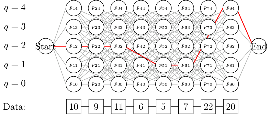
Despite initially seeming like a good idea, the restriction that we move an entire block of length \(L\) can lead to poor fits. Consider the following example sequence:
10 9 10 11 8 1000 999 1004 7 11 13 10It seems clear that there is a transition between an average of 10, to an average of 1000, back to an average of 10. With \(\nu=5\), we would expect something along the lines of:
2 2 2 2 2 200 200 200 2 2 2 2If, however, we analysed this sequence using the restrictions above with \(L=3\) and , then we would find something like the following:
2 2 2 60 60 60 120 120 120 2 2 2This is because we move the search window one base at a time (since we do not know when a transition might start – and in reality \(L\gg 1\), so making jumps of length \(L\) would wildly miss the beginning of transitions), and so we accidentally smooth over the transition edge, making the inference a disappointing compromise which meets neither set of data.
Once a transition has been accepted, we therefore perform an additional check, moving the start and end of the window around by a number of bases (up to some pre-specified fraction of \(L\)), searching for the exact location of the most likely beginning of the transition, and, given this more accurate model of where the transition begins, if there is a different value of \(q\) which should be assigned.
The end result is that it is indeed possible for the model to generate jumps from \(q_1 \to q_2 \to q_1\) where the total length of the \(q_2\) sequence is less than \(L\), seemingly changing the definition of \(L\) from the minimum transition size: however, the model must first be willing to move a block of width \(L\) for us to begin this more accurate search.